3.1. Functional Programming
Programming languages are often classified into one of several paradigms. For example, in imperative programming languages, computation is expressed as sequences of statements that update the state of the computation, including control flow statements like conditional and looping statements. In this context, “imperative” means “to give commands” (where statements are commands that are “given” in a program). Python is an imperative programming language, as are many others: C, C++, Java, etc.
We have also seen the object-oriented (OO) paradigm, where programs manipulate objects encapsulating some data (their attributes) and operations on the objects (their methods). Languages like Java are known as pure OO languages, because we must use classes and objects everywhere in our program. Python, along with C++ and others, is a multi-paradigm language: we can use OO features, but can stick with just imperative constructs if we like.
Another major paradigm of programming languages is the functional paradigm, in which functions are primarily used to compute values, rather than for their side effects (e.g., updating variables, printing). Functional programming languages include LISP, Scheme, Haskell, SML, and others. Python is not a pure functional language, but it does support a number of features commonly found in functional programming languages that are not traditionally found in languages like C, C++, Java, etc. (although some of these languages are starting to include features that are influenced by functional programming languages).
In this chapter, we will focus on two aspects of functional programming that Python supports: higher-order functions and anonymous functions.
3.1.1. Higher-order functions
Let’s say we wanted to find the value of an integral:
One way to do this is to apply integration rules, which tell us that the antiderivative of \(x^2\) is \(\frac{x^3}{3}\):
While it is possible to write a program that applies integration rules to evaluate a given integral, programs more commonly evaluate integrals using numerical methods, or ways to approximate the value of the integral.
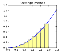
A common numerical method for computing integrals is the rectangle method, in which the area under the curve is approximated by \(N\) rectangles. If we are computing the integral between \(a\) and \(b\), then the width of each rectangle will be:
We can then approximate the integral as follows:
In other words, we divide the range between \(a\) and \(b\) into \(N\) subranges, all of width \(\Delta\). For each subrange, we compute the area of a rectangle, where the height of the rectangle is simply the value of the function at the midpoint of the subrange (using the start or end of the subrange is not desirable for reasons that are not worth getting into here) The sum of the areas of all those rectangles approximates the value of the integral between \(a\) and \(b\).
We can easily write a function that implements this approach. Let’s assume the function we’re integrating is the square function:
def square(x):
    return x ** 2
Our integration function, which simply implements the above summation
using a for loop, would look like this:
def integrate_square(lb, ub, N):
    '''
    Compute the integral of the square function between the
    specified bounds using the rectangle method.

    Inputs:
      lb (float): lower bound of the range
      ub (float): upper bound of the range
      N (int): the number of rectangles to use

    Returns (float): an approximation of the area under the curve
      between the specified bounds.
    '''

    delta = (ub - lb) / N
    sum = 0
    for i in range(N):
        sum += delta * square(lb + delta * (i + 0.5))
    return sum
If we run this function with N equal to 100, we get a reasonable approximation to
the expected value of the integral (\(2333.\overline{3}\))
>>> integrate_square(10.0, 20.0, 100)
2333.3250000000007
And, as we divide the area under the function into more rectangles, we get more accurate results, at the expense of more computation:
>>> integrate_square(10.0, 20.0, 1000)
2333.3332500000006
>>> integrate_square(10.0, 20.0, 10000)
2333.3333325000003
>>> integrate_square(10.0, 20.0, 100000)
2333.3333333249616
But what if we want to compute the integral of other functions? We would need to create functions that repeat essentially the same code! So, to integrate \(f(x)=2\cdot x\) we would have to write the following:
def double(x):
    return 2 * x

def integrate_double(lb, ub, N):
    '''
    Compute the integral of the double function between the
    specified bounds using the rectangle method.

    Inputs:
      lb (float): lower bound of the range
      ub (float): upper bound of the range
      N (int): the number of rectangles to use

    Returns (float): an approximation of the area under the curve
      between the specified bounds
    '''

    delta = (ub - lb) / N
    sum = 0
    for i in range(N):
        sum += delta * double(lb + delta * (i + 0.5))
    return sum
>>> integrate_double(10.0, 20.0, 10000)
299.9999999999999
If we compare integrate_square and integrate_double, we can
see that they are identical except for the call to the function
that is being integrated. In Python, and in most functional
programming languages, we address this code duplication by writing
a general purpose integrate function that, instead
of integrating a specific hard-coded function, takes
a function as a parameter:
def integrate(fn, lb, ub, N):
    '''
    Compute the integral of the specified function between the
    specified lower and upper bounds using the rectangle method.

    Inputs:
      fn (function): function to be integrated.  Must take a float
        and return a float
      lb (float): lower bound of the range
      ub (float): upper bound of the range
      N (int): the number of rectangles to use

    Returns (float): an approximation of the area under the curve
      (specified by the function parameter) between the bounds.
    '''


    delta = (ub - lb) / N
    sum = 0
    for i in range(N):
        sum += delta * fn(lb + delta * (i + 0.5))
    return sum
A call to this function looks like:
>>> integrate(square, 10.0, 20.0, 10000)
2333.3333325000003
Notice that integrate is nearly identical to both integrate_square
and integrate_double, except we have added a parameter called fn
that must be a function. When we call integrate, we are passing
the square function itself (not the result of calling square
with some specific values).
Because integrate takes a function parameter, we refer to it as
a higher-order function. A higher-order function is any function that takes
another function as a parameter or, as we’ll see later on, returns
a function as its result. Notice that we don’t define
higher-order functions in any special way; the syntax is the same as what
we’ve seen so far.
So, since the function to be integrated is now a parameter to integrate,
integrating a different function is as simple as calling
integrate with the function we want to integrate:
>>> integrate(double, 10.0, 20.0, 10000)
299.9999999999999
We can also use functions included with Python:
>>> import math
>>> integrate(math.sqrt, 10.0, 20.0, 10000)
38.54662833413495
Note that integrate will only work if we pass it a function that takes
a single float parameter and returns a float value. If we pass any other
type of function, our code will fail:
def multiply(a, b):
   return a*b
>>> integrate(multiply, 10.0, 20.0, 10000)
Traceback (most recent call last):
  File "<stdin>", line 1, in <module>
  File "<stdin>", line 21, in integrate
TypeError: multiply() missing 1 required positional argument: 'b'
The exact type of failure will depend on the function. In this case, for example, we passed a function with two required parameters where a function of one parameter was needed.
3.1.2. Anonymous functions
The integrate function can take a function as a parameter, but it
requires defining a separate function (like square and double)
to pass as a parameter. Instead of defining a function just for the
purposes of passing it as a parameter to another function, we can
instead use anonymous functions (also known as lambdas). An
anonymous function is basically a function we define on the fly
without using the def statement to give it a name. For example,
here is an anonymous function to compute the square of a single
parameter x:
lambda x: x ** 2
And here is an anonymous function to add two parameters x and y:
lambda x, y: x + y
The general syntax of an anonymous function is the following:
lambda <parameters>: <expression>
Notice that anonymous functions contain a single expression. They don’t
contain statements like a regular function (so you cannot use
conditional statements or loops), nor do they have a return statement. The
value the function will return is simply the result of the evaluating
the expression specified in the lambda using the values supplied
for the parameters.
And, since they’re anonymous, functions defined using lambda need
to be given a name before they can be called. Anonymous functions are
most commonly used as parameters to other functions. For example, the
following piece of code is equivalent to passing the square
function to integrate:
>>> integrate(lambda x: x ** 2, 10.0, 20.0, 10000)
2333.3333325000003
And the following piece of code is equivalent to passing the double function:
>>> integrate(lambda x: 2 * x, 10.0, 20.0, 10000)
299.9999999999999
3.1.3. map(), reduce(), filter()
Python provides a few very useful higher-order functions for working with lists.
Let’s say we had the following list:
lst = [1, 2, 3, 4, 5]
If we wanted to create a new list that contains the above values, but with each value incremented by one. We could do it like this:
lst2 = []
for x in lst:
    lst2.append(x + 1)
>>> print(lst2)
[2, 3, 4, 5, 6]
Functional programming languages provide a different mechanism
for processing lists in this way. In fact, most functional programming
languages lack looping constructs like for or while and, instead,
provide mechanisms to apply functions to sequences of values
in different ways (in the next chapter we will also see the general
mechanism that functional programming languages use to repeat operations: recursion)
For example, if we wanted to increment each value of the list by one, we would define a function that increments a single value:
def incr(x):
    return x + 1
Then, we would call that function on each value of the list, and
place the resulting values in a new list. However, instead of doing
this task with a for loop, we can do it with a single call to
the built-in map function
map(incr, lst)
The return value of this call is actually not a new list, but rather
an iterable object (like the kind of value that we get from a call to
range) that we can then use in a for loop or any other
context, such as a call to map, that requires an iterable, or
which we can convert to a new list:
>>> for x in map(incr, lst):
...     print(x)
...
2
3
4
5
6
>>> lst2 = list(map(incr, lst))
>>> lst2
[2, 3, 4, 5, 6]
As we saw with the integrate function, we don’t need to define
a new function before calling map and, instead, we can just
use an anonymous function as the first parameter to map:
>>> lst
[1, 2, 3, 4, 5]
>>> list(map(lambda x: x * 2, lst))
[2, 4, 6, 8, 10]
>>> lst
[1, 2, 3, 4, 5]
>>> list(map(lambda x: x ** 2, lst))
[1, 4, 9, 16, 25]
>>> lst
[1, 2, 3, 4, 5]
Notice that map does not change the list it operates on.
If we would like to create a new list with elements copied from an
input list only if they meet a given condition, we can instead use the
built-in filter function. This function takes a function that
returns a boolean result and a list as arguments. If, for a given
value in the list, the supplied function returns True, then the
value will be included in the resulting list. For example:
def is_odd(x):
    return x % 2 == 1
>>> lst
[1, 2, 3, 4, 5]
>>> list(filter(is_odd, lst))
[1, 3, 5]
Or, equivalently:
>>> list(filter(lambda x: x % 2 == 1, lst))
[1, 3, 5]
Another useful function found in many functional programming
languages is the reduce function. Unlike map and filter,
it does not apply a function to each value in the list; instead,
it repeatedly applies the function to reduce the list to a single value. For example, say we had
the following list:
lst = [1, 2, 3, 4]
If we wanted to multiply all the values in the list, we could write the following loop:
p = lst[0]
for x in lst[1:]:
    p = x * p

print(p)
24
Notice that this code boils down to evaluating this expression:
>>> ((lst[0] * lst[1]) * lst[2]) * lst[3]
24
If we define a multiply function, we could rewrite this expression
as follows:
def multiply(x, y):
   return x * y
>>> multiply(multiply(multiply(lst[0], lst[1]), lst[2]), lst[3])
24
And this repeated application of a function is exactly what reduce does:
>>> from functools import reduce
>>> reduce(multiply, lst)
24
Notice that unlike map and filter, reduce needs to be
imported from the functools library.
Or, using a lambda:
>>> reduce(lambda x, y: x * y, lst)
24
3.1.3.1. List comprehensions revisited
In Lists, Tuples, and Strings, we briefly described list comprehensions as shorthand notation for producing a new list based on an existing list. In particular, the following piece of code:
original_list = [1, -2, 3, 4, -5]
new_list = []

for x in original_list:
    if x > 0:
        new_list.append(x ** 2)

print(new_list)
[1, 9, 16]
Can be written more compactly using a list comprehension:
new_list = [x ** 2 for x in original_list if x > 0]
print(new_list)
[1, 9, 16]
Another way of thinking about list comprehensions is that they are a
more readable notation for combining a map and filter on a
list. The above list comprehension is equivalent to this code:
new_list = list(map(lambda x: x**2, filter(lambda x: x>0, original_list)))
print(new_list)
[1, 9, 16]
3.1.4. Returning a function
Recall that we defined higher-order functions as functions that can take other functions as arguments and return functions as results. So far, we’ve seen how higher-order functions can take a function as a parameter. In this section, we explain how to write functions that return new functions as results. For example, let’s say that, given an arbitrary function, \(f\) that takes a single float and returns a float, we want to compute a new function to give us the value of the derivative of \(f\) at a given point. In other words, the end result would look something like this:
def square(x):
    return x ** 2
>>> square(9)
81
>>> square_prime = derivative(square)
>>> square_prime(9)
18
Notice that the derivative function returns a function that we can
then call later in our code. square_prime is a variable, but one that refers
to a new function (instead of containing a value like an integer, or
referring to a list or dictionary). Furthermore, note that we want the
derivative function to work for any arbitrary function, so we
should also be able to write code like this:
>>> cube_prime = derivative(lambda x: x ** 3)
>>> cube_prime(3)
27
To explain how to do this, let’s start by explaining how we can compute the derivative of a single function. As we did with integration, we will compute the value of the derivative numerically.
The derivative of a function \(f\) at point \(x\) is its slope at that point. We can approximate the slope by computing the value \(f(x)\) and the value of the function at a nearby point \(f(x + dx)\):
In calculus, you consider the limit as \(dx\) goes to zero. Here we
will just assume \(dx\) is a small value like 0.00001.
So, if we had the following function:
def cube(x):
    return x ** 3
We could follow the above definition to define its derivative like this:
def cube_slope(x, dx=0.00001):
    '''
    Compute the slope of the cube function at the specified point.

    Inputs:
      x (float): point at which to evaluate the slope
      dx (float): difference (default: 0.0001)

    Returns (float): approximation to the slope of the cube
      function at the input point.
    '''

    return (cube(x + dx) - cube(x)) / dx
>>> cube(10)
1000
>>> cube_slope(10)
300.0002999897333
The derivate of \(x^3\) is \(3x^2\), so we are correctly approximating its slope (which would be 300 at \(x=10\)).
Now, if we wanted to compute the derivative for a different function, the resulting functions would look very similar:
def square(x):
    return x ** 2

def square_slope(x, dx=0.00001):
    '''
    Compute the slope of the square function at the specified point

    Inputs:
      x (float): point at which to evaluate the slope
      dx (float): difference (default: 0.0001)

    Returns (float): approximation to the slope of the square
      function at the input point.
    '''

    return (square(x + dx) - square(x)) / dx
One first approach at generating this code could be to create a
general purpose slope function, like we did with our integration
function:
def slope(f, x, dx=0.00001):
    '''
    Compute the slope of the specified function at the specified
    point

    Inputs:
      f (function): function to take the slope of.  The function
        must a float and return a float
      x (float): point at which to evaluate the slope of f.
      dx (float): difference (default: 0.0001)

    Returns (float): approximation to the slope of the specified
      function function at the input point.
    '''

    return (f(x + dx) - f(x)) / dx
>>> slope(cube, 10)
300.0002999897333
>>> slope(square, 10)
20.00000999942131
However, we actually want to generate new functions (so we don’t have to pass
cube or square as a parameter every time we want to compute its derivative).
We do this by defining
one function inside another function, and having the outer function return
the inner function:
def derivative(f):
    '''
    Create a function of one variable that computes the derivative
    of the specified function.

    Inputs:
      fn (function): function to be differentiated.  Must take a
        float and return a float

    Returns: a function that computes the derivative of the
      specified function at a given point with an optional
      parameter for dx.
    '''

    def slope(x, dx = 0.00001):
        ''' Compute the slope of f at the specified point '''

        return (f(x + dx)-f(x)) / dx

    return slope
In this case slope, the inner function, is the function we want to generate.
Notice that it does not need to take a function as a parameter. Instead, because it
is in the same scope as the parameter f, it can access f directly. The outer
function, derivative, takes a function parameter and will return a slope
function that will use that function to compute the slope.
>>> cube_prime = derivative(cube)
>>> cube_prime(2)
12.000060000261213
>>> cube_prime(5)
75.00014999664018
>>> cube_prime(5, dx=0.0000001)
75.00000165805432
>>> quad_prime = derivative(lambda x: x ** 4)
>>> quad_prime(3)
108.0005400012851
Because the derivative of a function of one variable, is itself a function of one variable, we can apply our derivative function repeatedly to get functions that compute the second derivative, third derivative, etc.
>>> cube_prime = derivative(cube)
>>> cube_double_prime = derivative(cube_prime)
>>> cube_triple_prime = derivative(cube_double_prime)
>>> cube_prime(10)
300.0002999897333
>>> cube_double_prime(10)
59.99936547596007
>>> cube_triple_prime(10)
227.37367544323203
3.1.5. Scoping and inner functions
Before we move on to our next topic, recursion, let’s revisit the
topic of scoping. Recall that every variable is defined and
accessible within a specific part of the program, known as the variable’s scope.
Our earlier discussion (see Variable scope) covered local variables,
which have scope that is local to a specific function and global
variables, which are defined outside the context of any function.
Adding inner functions to the mix introduces in a third kind of scope:
nonlocal. A local variable or parameter in an outer function, such
as the parameter f in our derivative function, is visible as a
nonlocal variable in an inner function as long as it is not shadowed
by a variable or parameter of the same name in the inner function.
Like globals, nonlocal variables are read-only within an inner
function unless the programmer explicitly declares them as
nonlocal.